Detection of phishing websites is a really important safety measure for most of the online platforms. So, as to save a platform with malicious requests from such websites, it is important to have a robust phishing detection system in place.
Thanks to people like, Rami M. Mohammad, Fadi Thabtah, and Lee McCluskey who have worked intensively in this area. In this post, we are going to use Phishing Websites Data from UCI Machine Learning Datasets. This dataset was donated by Rami Mustafa A Mohammad for further analysis. Rami M. Mohammad, Fadi Thabtah, and Lee McCluskey have even used neural nets and various other models to create a really robust phishing detection system. I really encourage you to have a look at the original papers here and here.
For this very basic analysis, we are going to use multiple models, and see which one fits the best with our dataset. And finally, the most important part - a breakdown of most important features to detect a phishing website using a randomForest Fit.
We’ll start with loading the csv file, in our R Script and setting the new column names.
1
2
3
4
5
6
7
8
9
10
11
12
13
14
15
16
17
18
19
20
21
22
library(caret)
library(doMC)

# Register 4 cores for parallel computing
registerDoMC(4)

# Read the data from csv file
data <- read.csv('Datasets/phising.csv', header = F,
				colClasses = "factor")

# Names list for the features
names <- c("has_ip", "long_url", "short_service", "has_at",
		   "double_slash_redirect", "pref_suf", "has_sub_domain",
		   "ssl_state", "long_domain", "favicon", "port",
           "https_token", "req_url", "url_of_anchor", "tag_links",
           "SFH", "submit_to_email", "abnormal_url", "redirect",
           "mouseover", "right_click", "popup", "iframe",
           "domain_Age", "dns_record", "traffic", "page_rank",
           "google_index", "links_to_page", "stats_report", "target")

# Add column names
names(data) <- names
Here we are importing caret and doMC libraries and then registering 4 cores for parallel processing. You can set the number of cores according to your machine.
All of the features in this dataset are factors, that’s the reason I have used colClasses = "factor" in read.csv method. You can have a look at the README.md file in this Github Repo, to get an overview of the possible values of each feature.
Now, first thing first, let’s have a look at the data,
1
str(data)
'data.frame':	2456 obs. of  31 variables:
 $ has_ip               : Factor w/ 2 levels "0","1": 2 1 1 ...
 $ long_url             : Factor w/ 3 levels "0","1","-1": 2 2 1 ...
 $ short_service        : Factor w/ 2 levels "0","1": 1 1 1 ...
 $ has_at               : Factor w/ 2 levels "0","1": 1 1 1 ...
 $ double_slash_redirect: Factor w/ 2 levels "0","1": 2 1 1 ...
 $ pref_suf             : Factor w/ 3 levels "0","1","-1": 3 3 3 ...
 $ has_sub_domain       : Factor w/ 3 levels "0","1","-1": 3 1 3 ...
 $ ssl_state            : Factor w/ 3 levels "0","1","-1": 3 2 3 ...
 $ long_domain          : Factor w/ 3 levels "0","1","-1": 1 1 1 ...
 $ favicon              : Factor w/ 2 levels "0","1": 1 1 1 ...
 $ port                 : Factor w/ 2 levels "0","1": 1 1 1 ...
 $ https_token          : Factor w/ 2 levels "0","1": 2 2 2 ...
 $ req_url              : Factor w/ 2 levels "1","-1": 1 1 1 ...
 $ url_of_anchor        : Factor w/ 3 levels "0","1","-1": 3 1 1 ...
 $ tag_links            : Factor w/ 3 levels "0","1","-1": 2 3 3 ...
 $ SFH                  : Factor w/ 2 levels "1","-1": 2 2 2 ...
 $ submit_to_email      : Factor w/ 2 levels "0","1": 2 1 2 ...
 $ abnormal_url         : Factor w/ 2 levels "0","1": 2 1 2 ...
 $ redirect             : Factor w/ 2 levels "0","1": 1 1 1 ...
 $ mouseover            : Factor w/ 2 levels "0","1": 1 1 1 ...
 $ right_click          : Factor w/ 2 levels "0","1": 1 1 1 ...
 $ popup                : Factor w/ 2 levels "0","1": 1 1 1 ...
 $ iframe               : Factor w/ 2 levels "0","1": 1 1 1 ...
 $ domain_Age           : Factor w/ 3 levels "0","1","-1": 3 3 1 ...
 $ dns_record           : Factor w/ 2 levels "0","1": 2 2 2 ...
 $ traffic              : Factor w/ 3 levels "0","1","-1": 3 1 2 ...
 $ page_rank            : Factor w/ 3 levels "0","1","-1": 3 3 3 ...
 $ google_index         : Factor w/ 2 levels "0","1": 1 1 1 ...
 $ links_to_page        : Factor w/ 3 levels "0","1","-1": 2 2 1 ...
 $ stats_report         : Factor w/ 2 levels "0","1": 2 1 2 ...
 $ target               : Factor w/ 2 levels "1","-1": 1 1 1 ...
So, we have some 30 features and a target variable with two levels(1, -1), i.e. whether a website is a phishing website or not.
We’ll now create a training and test set using caret’s createDataPartition method. We’ll use test set to validate the accuracy of our detection system.
1
2
3
4
5
6
7
8
9
# Set a random seed so we can reproduce the results
set.seed(1234)

# Create training and testing partitions
train_in <- createDataPartition(y = data$target,
						p = 0.75, list = FALSE)

training <- data[train_in,]
testing <- data[-train_in,]
Now, we are ready to try a few models on the dataset. Starting with a Boosted logistic Regression model. Let’s see how that perform on our quest for the nearly perfect phishing detection system ;).
1
2
3
4
5
6
7
8
9
10
11
12
13
14
15
################ Boosted Logistic Regression ################

# trainControl for Boosted Logisitic Regression
fitControl <- trainControl(method = 'repeatedcv', repeats = 5,
                           number = 5, verboseIter = T)

# Run a Boosted logisitic regression over the training set
log.fit <- train(target ~ .,  data = training,
				method = "LogitBoost", trControl = fitControl,
				tuneLength = 5)

# Predict the testing target
log.predict <- predict(log.fit, testing[,-31])

confusionMatrix(log.predict, testing$target)
We are using caret’s trainControl method to find out the best performing parameters using repeated cross-validation. After creating a confusion Matrix of the predicted values and the real target values, I could get a prediction accuracy of 0.9357, which is actually pretty good for a Boosted Logistic Regression model.
But of course we have better choices for models, right? And there is no reason, for not using our one of the most favourite SVM with an RBF Kernel.
1
2
3
4
5
6
7
8
9
10
11
12
13
14
15
################## SVM - RBF Kernel ####################

# trainControl for Radial SVM
fitControl = trainControl(method = "repeatedcv", repeats = 5,
						 number = 5, verboseIter = T)

# Run a RBF - SVM over the training set
rbfsvm.fit <- train(target ~ .,  data = training,
					method = "svmRadial", trControl = fitControl,
					tuneLength = 5)

# Predict the testing target
rbfsvm.predict <- predict(rbfsvm.fit, testing[,-31])

confusionMatrix(rbfsvm.predict, testing$target)
Woah! I am getting a 0.9706 accuracy with a SVM and RBF Kernel. Looks like there is almost no escape for phishing websites now :D.
But, since one of the most important reason I picked up this analysis was to find out the most important predictors, that can identify a phishing website, we’ll have to move to Tree-based models to get the variable importance.
So, let’s fit a Tree bagging model on our dataset.
1
2
3
4
5
6
7
8
9
10
11
12
13
14
################## TreeBag ###################

# trainControl for Treebag
fitControl = trainControl(method = "repeatedcv", repeats = 5,
						 number = 5, verboseIter = T)

# Run a Treebag classification over the training set
treebag.fit <- train(target ~ .,  data = training,
					 method = "treebag", importance = T)

# Predict the testing target
treebag.predict <- predict(treebag.fit, testing[,-31])

confusionMatrix(treebag.predict, testing$target)
Now, this is something, an accuracy of 0.9739 and we also get our variable importances :).
But I am not going to show that, without fitting another tree model, the almighty(throw-anything-at-me) Random Forests.
1
2
3
4
5
6
7
8
9
10
11
12
13
14
15
####################### Random Forest ########################

# trainControl for Random Forest
fitControl = trainControl(method = "repeatedcv", repeats = 5,
						 number = 5, verboseIter = T)

# Run a Random Forest classification over the training set
rf.fit <- train(target ~ .,  data = training, method = "rf",
                     importance = T, trControl = fitControl,
                     tuneLength = 5)

# Predict the testing target
rf.predict <- predict(rf.fit, testing[,-31])

confusionMatrix(rf.predict, testing$target)
That’s some coincidence(or-not), with mtry = 21, we are still getting an accuracy of )0.9739 with our Random Forest model, which is actually pretty good, even for practical purposes. so, finally let’s have a look at the variable importances of different features,
1
plot(varImp(rf.fit))
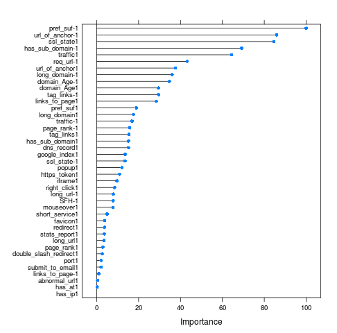
According to our Random Forest model, 10 of the most imporant features are:
		* pref_suf-1           100.00
		* url_of_anchor-1       85.89
		* ssl_state1            84.59
		* has_sub_domain-1      69.18
		* traffic1              64.39
		* req_url-1             43.23
		* url_of_anchor1        37.58
		* long_domain-1         36.00
		* domain_Age-1          34.68
		* domain_Age1           29.54
Numerical values suffixing the features name are just the level of the factor of that particular feature. As apparent from this variable importance plot and from our own intuition, features listed here are indeed some of the most important attributes to find out whether a given sample is a phishing website or not.
Like, if there is prefixes or suffixes being used in the url then there are very high chances that it’s a phishing website. Or a suspicious SSL state, having a sub domain in url, having a long domain url, etc. are actually really important features that can clearly identify a phishing website.
One can create a phishing detection system pretty easily if he/she can get the information about these predictors. Rami M. Mohammad, Fadi Thabtah, and Lee McCluskey have also mentioned in their original paper, how they did it.
I am sure that neural nets can further increase the accuracy of phishing detection system, but I tried to do a very basic analysis and it worked out pretty good. But of course getting and filtering out the data, creating factors out of different attributes is probably the most challanging task in phishing website detection.
You can further look at the Github repo with the above code at: rishy/phishing-websites. Your feedbacks and comments are always welcomed.